There is a special case of element, where the determinant of the Jacobian is "allowed" to be zero. This element is called the crack tip element, and is basically a quadratic quadrilateral element where two of the mid nodes are placed strategically in order to give a zero determinant at the corner node in between.
You can basically calculate the distance yourself, simply set up the trial function for the position, then differentiate to get the Jacobian and solve the determinant for zero at one of the corner nodes. It is actually a fun little exercise! If you calculate the length, you will note, that the resulting distance is 1/4 of the edge length - the undeformed element has the mid node at 1/2 the edge length.
But what does all this mean and can we do with this now? The determinant of the Jacobian effectively gives the volume (area) change for a given infitisimal point. That means, if det(J) equals 1, we have no change. If it is 2, we have an 100% increase. However, if it is zero, we produced a singularity, meaning we compressed everything into a point with no radius - even our infitisimal point gets even smaller. This zero determinant is the same concept of a division by zero. We can actually get a value from such a division, for example by looking at the limit at infinity. But back to our crack tip. The idea of the crack tip, as far as I understood it, is to model the emerging front of a crack where the material gets discontinuous. But as we can not really model discontinuity in the mesh, we use the singularity to model the stress concentrations at the point. By using an element where a single node gives a determinant of zero, allows us to model the diverging stress curve at that point, i.e. we can model a theoretical infinite stress.
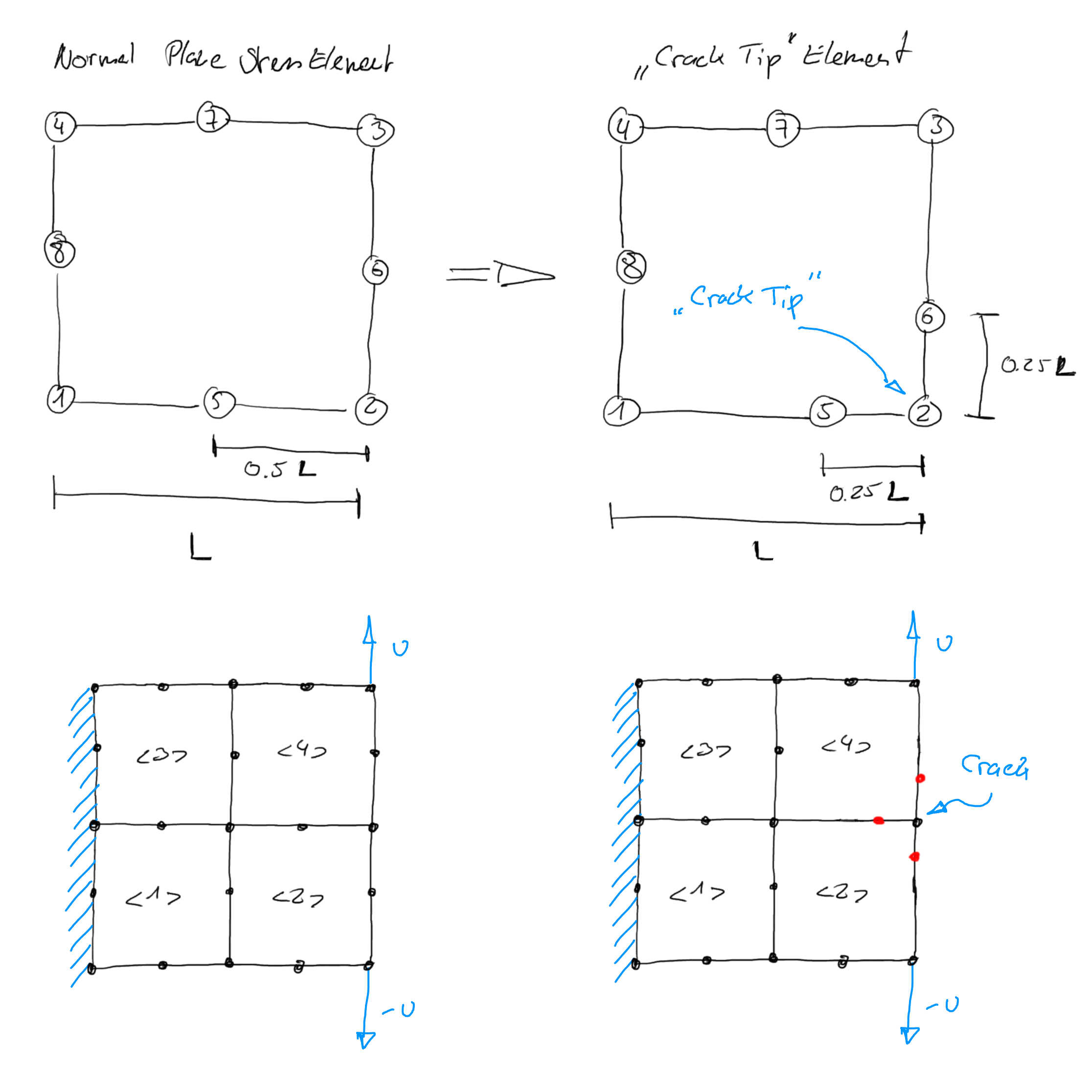
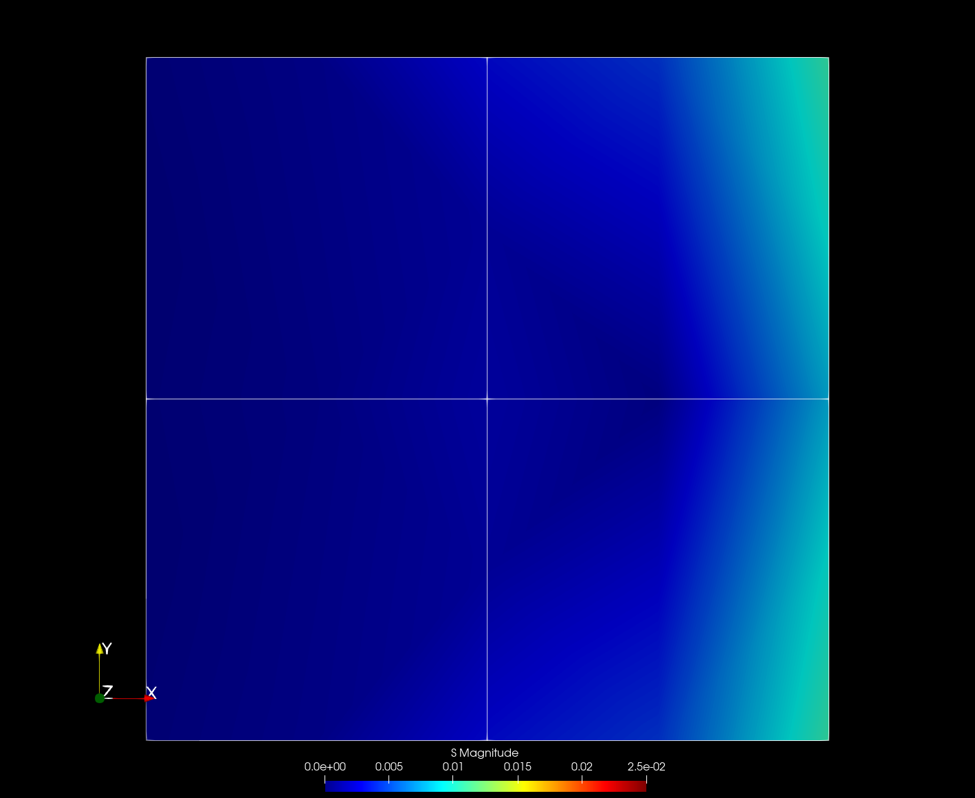
Let us look at this example in more detail using calculix to calculate some numbers. First, we create a normal mesh using four CPS8 elements. We fix them on one side and apply a displacement at the two corner nodes the opposite side, effectively loading the elements in tension. We can probably already guess what will happen: The stress will be highest at the two corner nodes and gradually decrease towards the center from both sides. Indeed, we see the same in the output:
But, what happens if we introduce the crack at the middle between the two nodes? We apply the moved nodes and run the simulation again:
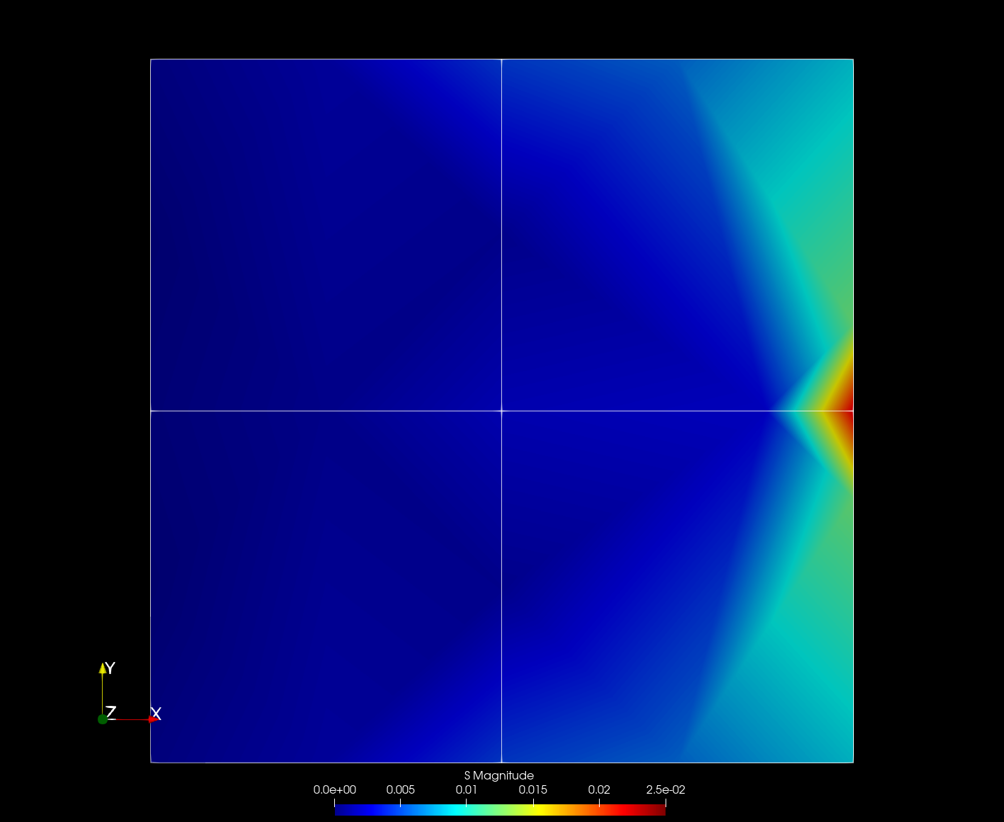
We can immediately see the stress concentration in the middle. If we plot the stress along the edge, we can see this more clearly:
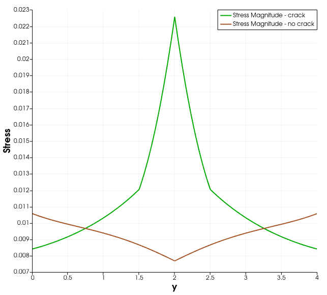
But wait! Why is the stress not infinity, as proposed by the limit when we set the determinant to zero? The reason is the numerical model we use. First of all, we are solving the differntial equations here at the integration points and then transforming the result back onto the nodes. You can see what that means if you switch from CPS8 to CPS8R elements, which use only a single integration point. In that case, we do not even see the singularity that easily! In the end, our finite element model is just a model - which has obviously some drawbacks. If you look carefully at the element stress distribution, you can also see where the interpolation comes from - for example you can see some diagonal lines forming between the mid-nodes.
So we see, that we can use such elements to model stress concentrations without actually meshing the discontinuity, for example by inserting many many small elements at the crack tip. On the other hand this also gives a nice example, what happens if the mesh quality is bad and for some reason we introduce such distorted elements into our mesh! In such a case, we would see high stress concentrations at points where we do not have them in the real world.
If you want to play around with the two models, here are the input decks for download: